Isolated EPA Per Play: Evaluating NFL Quarterbacks

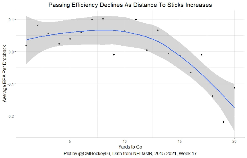
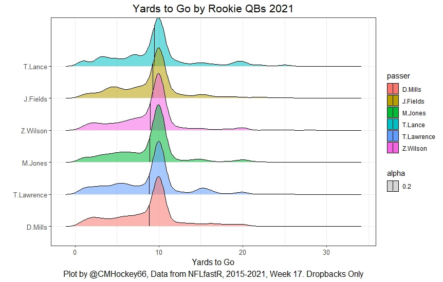
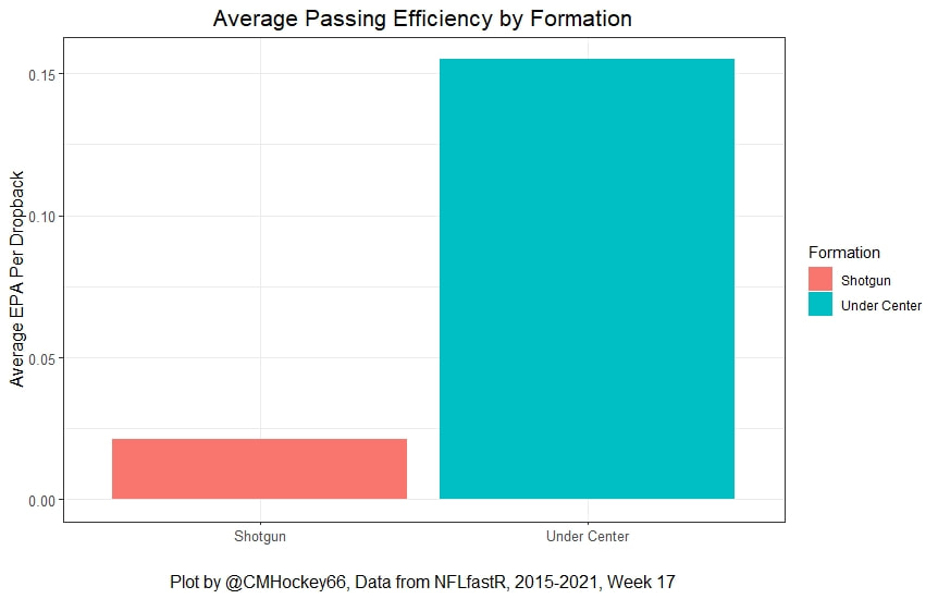
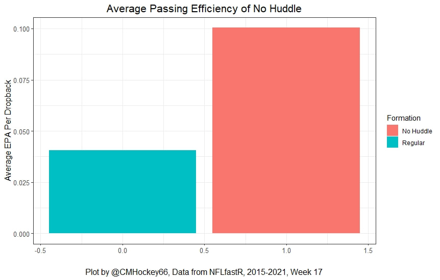
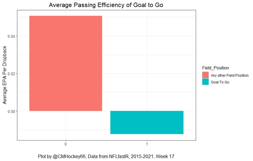
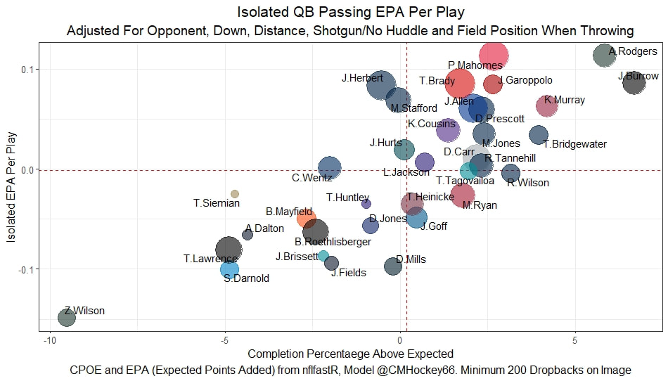
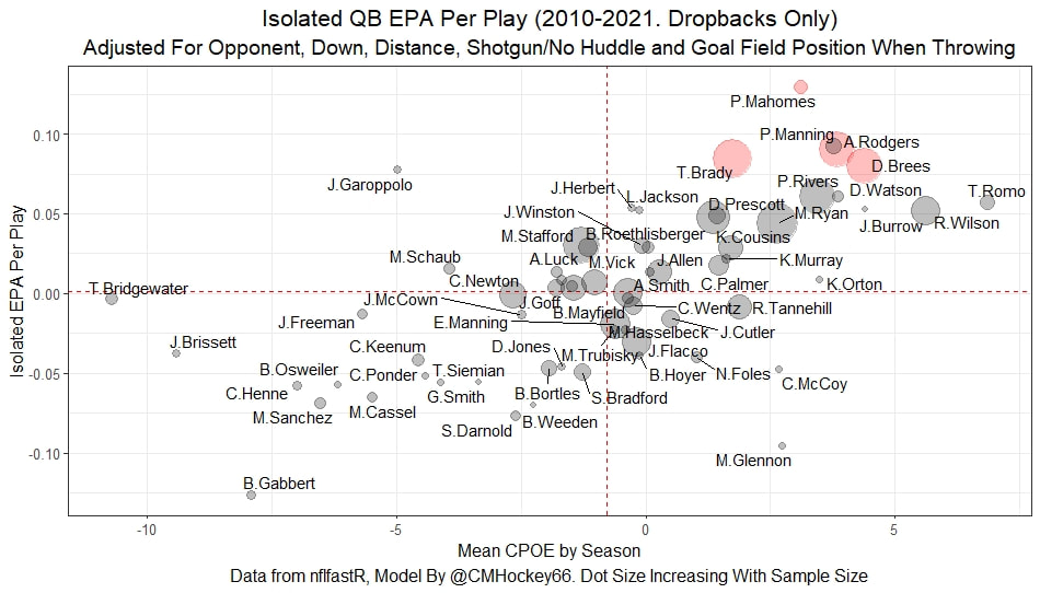
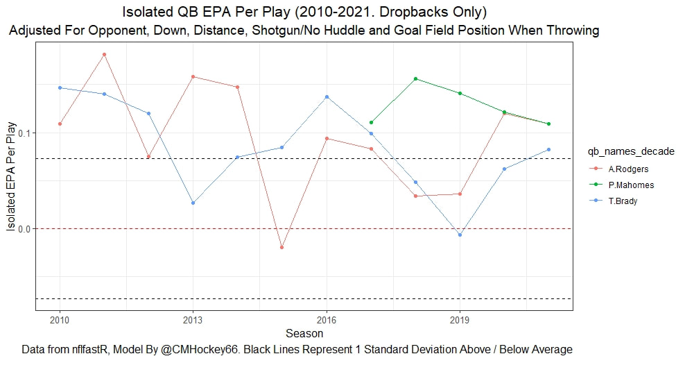
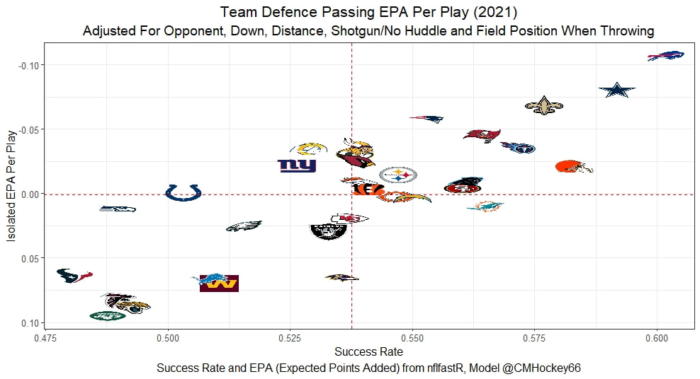
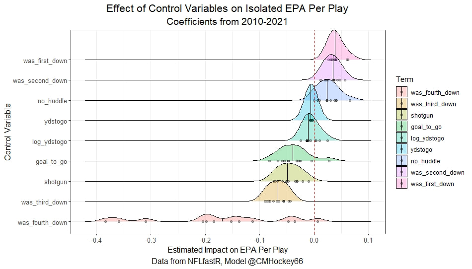
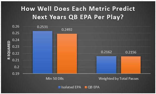
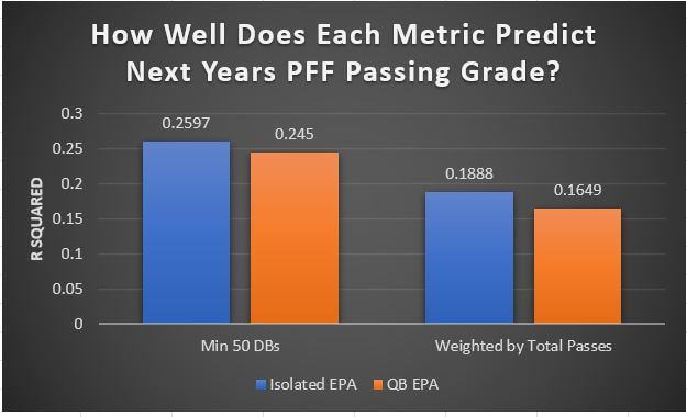
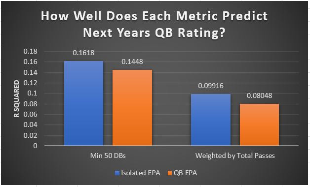
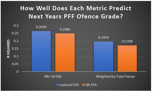
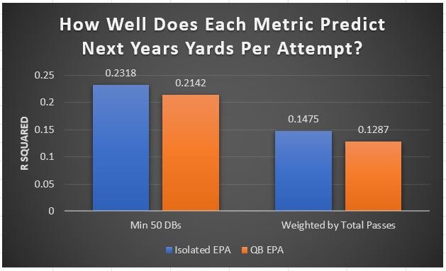
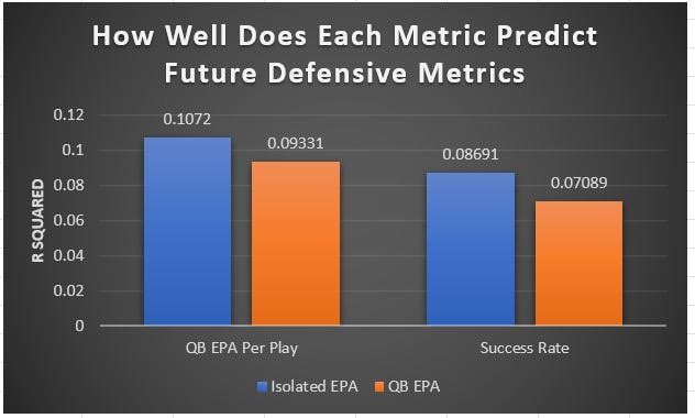
I have previously written about turnover adjustments to Expected Points Added (EPA) per play. This is because I generally use EPA to evaluate quarterbacks. As a result, I do not believe an ideal EPA statistic should penalize QBs for things out of their control. Today, we are going to expand on that philosophy. We are going to introduce my Isolated EPA Per play model fully. This ridge regression model aims to better evaluate QB's effect on EPA per play by accounting for various contextual factors they cannot control. Note that since this post is about evaluating NFL quarterbacks better, everything from here on in will be about plays labelled as QB dropbacks in the NFLfastR dataset.

Theory
This methodology comes from my first favorite sport, Hockey. When scrolling through NFL Twitter, I noticed a familiar theme. Football people sometimes filter out "garbage time". These charts only used stats while the game is at least somewhat close. The theory is that stats when up 37 points aren't super meaningful. Hockey analysts noticed a similar problem some time ago. These analysts coined the term "score effects". Winning teams get outplayed in hockey once winning.

Originally, "Corsi close" was used to get around this. Corsi close only used player statistics when the score was within a few goals. But, what hockey analysts have done since is "score adjust". They have found that rather than filtering out good some of our precious data, it is better to adjust for these variables, generally using regression models. No amount of math can make up for the lack of data, so I believe this change is very important. Then hockey analysts started doing this for all sorts of variables. For example, RAPM, the ridge regression model that inspired this post, doesn't punish players for the quality of their competition/ teammates, zone starts, score effects, etc.

So I figured something along the same lines could be done for Football. Instead of filtering out data, it is preferable properly adjust for the contextual variables that influence statistics like EPA. To make such an adjustment, I decided to make a ridge regression model. This would allow us to estimate all of the quarterback's and defense's effects on EPA that season, independent of each other and various contextual variables we know affect outcomes. For example, if one team doesn't throw enough on early downs (when it's relatively easy to throw), the QB's raw EPA numbers will be punished, but this model will account for this. Not punishing QBs for coaching decisions should QB evaluations with EPA. Now let's dive into the model.​

Public Code For Open Source Changes
Now we know where I got the idea for this model. I want to note that I am not an NFL football expert. Somebody with far more domain knowledge than me may be better at picking control variables than me. This is why I have made the code for this public. Not only that, but I published the code to make this model public going back ten years (if you want, you could easily run it farther back) and attached code at the end to allow for year-over-year testing of the model in case anyone wants to try and evaluate their improvements. So don't think this model is something I think is final; you are welcome to take a crack at the code, too; if you think I'm missing something (I probably am) or overfitting somewhere, please improve what I have done. The code for this post can be found here.

Control Variables
So, let's start with how the model's control variables affect EPA per play. Let's begin with the easiest one, down.

Down
A major piece of the NFL analytics movement has suggested that NFL offences should pass more on early downs. Why? Well, passing is more efficient than running, on average, but there is more to the story. It has been easier to pass the earlier the down for as long as we have data. This gives an edge for smart teams to maximize passing efficiency by passing more early.  This edge adds a layer to QB evaluation. If not every QB passes an equal amount on every down, and different downs have different difficulties, it is one-way teams can make passing easier/more difficult on their QB.  There are massive differences across the league too.

Since play calling is not in the QB's job description (I understand they can manipulate these things to some degree, but still), it does not make sense to penalize a QB whose team forces him to pass on later downs more often. To account for this in the model, 4 dummy variables have been created. One variable for each down. One of these variables will be equal to one at any given time, depending on the down. For example, if a QB passes on second down, the second down variable will be equal to one, while the 1st, 3rd and 4th down variables would all be equal to 0.

Distance (Yards to Go).
The following control variable is the distance to the sticks. In other words, how many yards the QB needs to gain to get a first down on that drop back. Thus resetting the number of plays, they have to gain another first down.  Again, as distance increases, it becomes more and more difficult to generate positive plays.

Again this creates a problem because QBs pass at different distances over the course of a season. For example, let's follow the rookie QBs as our case study.

Trey Lance has had the longest average yards to go, while David Mills is on the opposite side of the spectrum. While these differences are not massive, Mills's average yards to go is over half a yard shorter than Lance's. Half a yard over hundreds of pass attempts adds up. QBs, of course, have some control over this. But again, play calling is not in the job description. So it doesn't make sense to penalize QBs who are asked to pass from longer distances. It's also worth noting that there is an evident nonlinearity.  To account for this, the yards will go variable, and a logged transformation of the variable will go into the model.

Shotgun
Next up we have the shotgun variable. This is a dummy variable set equal to one if the QB lined up in the shotgun instead of under center. This probably matters because teams tend to pass more from the shotgun than under center. While they tend to run more from under center than the shotgun. NFL defenses know this and adjust accordingly. These adjustments are likely what makes passing out of the shotgun so tricky.

Passing from under center has been about six times more efficient than passing from the shotgun. The difference above almost certainly has a lot to do with play action. Play action rates are also almost certainly much higher from under center than the shotgun because teams can more credibly threaten a run play. The run and play-action rate is likely much of the reason for this effect. Continuing our common theme here, QBs have limited to no control over where they line up since they don't call or create plays. So it would be unfair to penalize QBs whose offences ask them to pass out of the shotgun more often.

No Huddle
After shotgun, we have another dummy variable, no-huddle. This dummy variable equals one when the team hurries and does not huddle between plays. This makes it difficult for the defences to make adjustments and leads to more efficient passes.

Goal to Go
The final control variable in the model is also a dummy variable. This time it is set equal to one when the team is in goal to go. This means they cannot gain any more first downs because the drive started within 10 yards of the end zone. The only positive outcome here is scoring, you can't get a fresh set of downs and continue on. No matter what happens on these drives, the possession will change after a maximum of 4 downs. This probably matters in the model because of something that any experienced Madden player will know. As you approach the goal line, there is less and less space for the pass defense to cover. As a result, passing in goal-to-go is really, really difficult in goal-to-go situations.

Goal to go will go in the model the same way as the two dummy variables above.

Opponent Adjustment
The final control variable to evaluate the QBs will be an opponent adjustment. Not all teams have equally good defences. Passing against the 2021 Bills or Patriots has been very difficult. Teams have averaged negative expected points against them this season. On the contrary, specific teams like the Jaguars and have bled points to their opponents. So there will finally be a control variable for the team the QB was passing against in the model. Again this will be done with dummy variables set equal to one corresponding to which defence the QB was passing against on that play.
Another benefit of this is that we will obtain estimates of team pass defence along with QB estimates. Since the QBs also go into this model, the pass defence estimates will be isolated from the QB they are playing, along with all the control variables listed above. As I write this, I wonder if a model like this is more beneficial for defences than QBs because it is usually assumed that even a great defence is mainly at the mercy of the QB they are facing.


Target Variable
Now we can move to the model's target variable. I will be using a variation of QB EPA from NFLfastR. QB EPA is a modified version of EPA. QB EPA doesn't punish QBs for expected points lost on receiver fumbles. Similarly, my turnover-adjusted EPA discussed here (link here) will be the target variable. This treats all fumbles and interceptions as having their average EPA for that year rather than their actual impact. For example, the average fumble cost a team 2.5 expected points in 2021. But, a QB may get lucky and have their team recover said fumble and gain points on that fumble. Or another QB can lose 7+ expected points on the exact same play if the other team recovers for a touchdown.

In the EPA used in this model, the QB will be punished 2.5 points no matter the outcome. I did this because the model aims to estimate how a QB has influenced EPA per play, and the article linked above shows evidence fumbling or throwing picks in high/low EPA situations is not a skill. The goal of this model is to evaluate Quarterbacks. So if the mitigating expected points lost on a per fumble or interception basis is not a skill, I do not believe there is any reason to include it in our analysis. There is no reason to add randomness to QB evaluations if we do not have to. So fumbles and interceptions will all have the same effect on EPA in this model, no matter the outcome. Again if you believe this was a mistake, the code is public! Take a shot at the estimation without this adjustment if you wish

How QBs Enter the Model
We can now add QBs to the model with all the control variables. The QBs go into the model as dummy variables. Each QB has their own variable set equal to one if they are the one dropping back to pass. The model then estimates how that variable (the QB) affects EPA per play independent of all the other variables in the model. This is how we use regression to isolate QBs from contextual variables.


Why Ridge Regression?
For this analysis, Ridge regression is used in hockey instead of Ordinary Least Squares (OLS) for two main reasons. I will be following the same idea here. The first Ridge regression is preferable to OLS is that Ridge regression (which penalizes the coefficients by some lambda) tends to deal better with collinearity. So if the model is being estimated early in the season and some QB estimates are pretty colinear with the defence, ridge regression should be preferable here.

​Additionally, ridge regression allows a coefficient to be estimated for each dummy variable-based coefficient. This way, we get an estimate for how much each quarterback, down and defence affected dropback EPA that season. If we used OLS, one quarterback, one defence, and one down would all be dropped from the model, and the interpretation would be increasingly difficult, especially year over year.
QB ResultsNow for the fun and exciting part. Once we have a model to quantify QB performance independent of various contextual factors they do not control, we can better isolate QBs from their surroundings. So we can plot all NFL QBs isolated EPA Per dropback in 2021.

We can see Patrick Mahomes and Aaron Rodgers leading the way atop the list. Right behind them is Joe Burrow. Burrow only ranked 7th in EPA per pass, but the adjustments shot him up the list. We can also view these results over a more extended time period. For example,  we can estimate the most efficient QBs on a per-play basis since 2010.

It's no surprise Patrick Mahomes sits far above everyone else. Those next closest behind him include a group of many of the best ever to play, Payton Manning, Aaron Rodgers, Tom Brady and Drew Brees. Additionally, we can even view these estimates over time. Here are some of the all-time greats isolated EPA per play estimates over the years. Remember all of this is in the code so you can play around with evaluating different quarterbacks over time if you wish! Go to line 4500 in the R code if you wish to make your own plots with different players selected

Defensive Results
As I mentioned earlier, we can also use this to evaluate defenses too. Here are the top defensive teams from the previous season!

Effect of Control VariablesTo better understand the estimates above, we can re-visit the control variables. This time we can look at how the control variables affect EPA per play independent of the QBs and other control variables. This is something the graphs above did not do. Here are the distributions of each variable from the past 11 seasons in the model.

​All the variables mostly show the same sign as directed. For example, it's more challenging to pass the later down and is tough to pass into the end zone etc. These estimates help illustrate how much easier it is to pass in these specific situations. Again I am not an expert here, but it is encouraging the signs of the control variables do not flip very often. A control variable that did not influence EPA per play would theoretically be fluctuating around zero, which does not appear to be happening generally.  If you think i missed something here, feel free to update the model!

Year Over Year Testing 
The last order of business when introducing a new player evaluation model is to test it against other publicly available QB evaluation metrics. First up let's compare the year over year relationship between my new Isolated EPA and future EPA Per play. We will be using regular QB EPA per play as the benchmark here. Note the weighted by total passes will also only include QBs who had at least 50 drop backs to avoid super small samples.

While nothing crazy has been done here and the differences are not worth bragging about, Isolated EPA is definitely not a worse predictor of future QB EPA per play than past QB EPA per play. This is encouraging, and the general trend holds when evaluating this metric against other metrics. Note the next metrics all came from PFF which I downloaded. This is the only part of this post that won't be publicly available because I can't post other peoples data. Note the PFF data I used was from 2014-2020 because I did this mid season. 

This time the difference is slightly large. Isolated EPA per play has been ever so slightly more predictive of future PFF passing grade than QB EPA per play. More encouraging results! The next three metrics will be presented together to show a similar trend. I know these make less sense to test against but I wanted to include them simply because they were in the PFF dataset downloaded anyways, and show the same general trend robust across more QB evaluation metrics. 

The general trend here is pretty similar. This new metric is somewhere between equally as and more predictive of public metrics used to evaluate QBs than previous QB EPA per play. While this may not be the best way to evaluate a new metric, it's a good sign.

We can also compare the relationship on the defensive side of the football. It turns out the Isolated EPA numbers are more predictive of future QB EPA per play allowed by defences than past QB EPA per play allowed by defences.

There is a similar trend on the defensive side of the football. While the differences are not huge, this new metric predicts future EPA per play allowed and success rate better than past EPA per play! I do not believe this metric is perfect, and people who know football better than me may easily be able to improve it. However I believe the general logic makes sense, and testing results are encouraging.