Isolated EPA Per Play

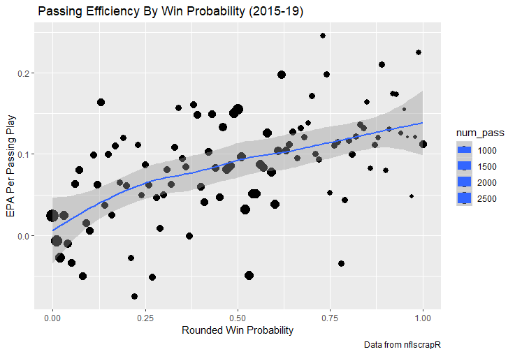
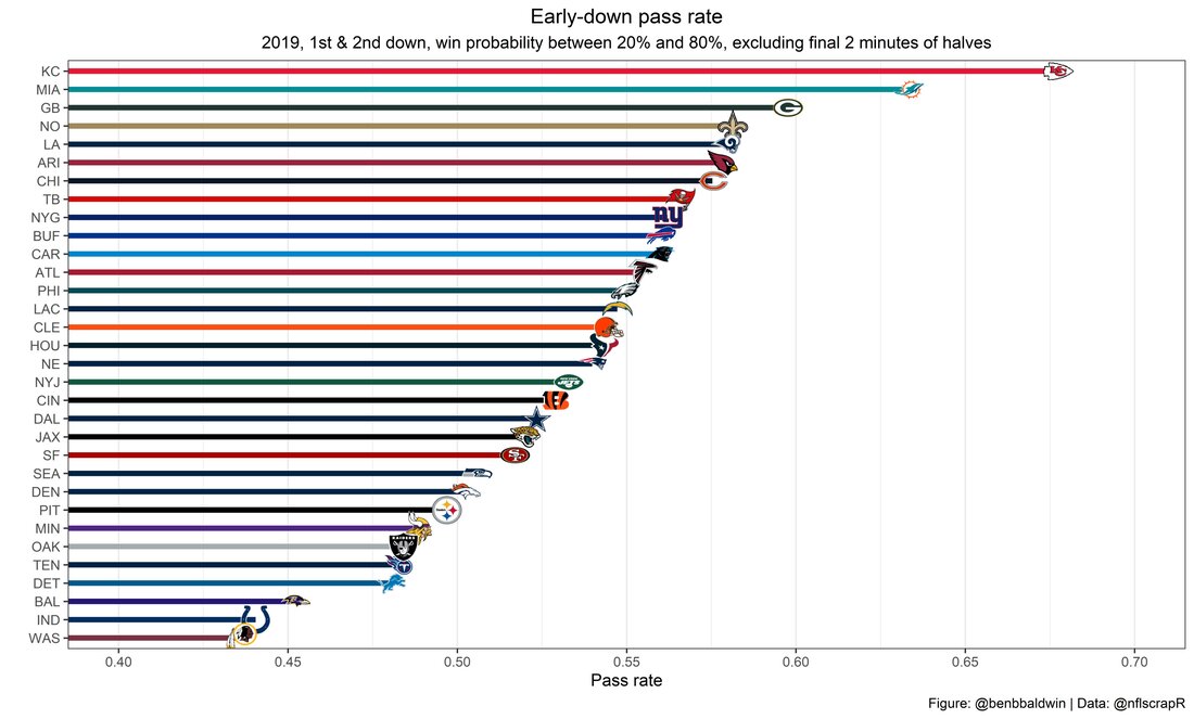
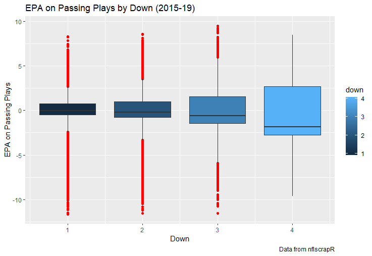
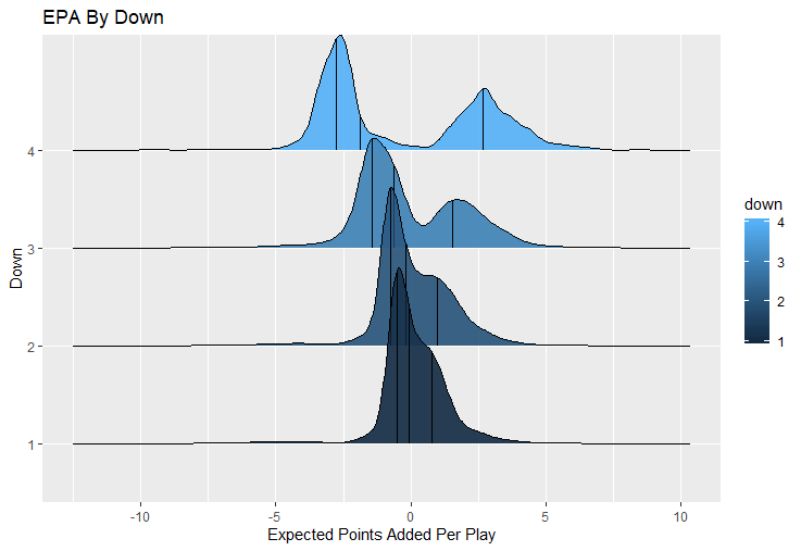
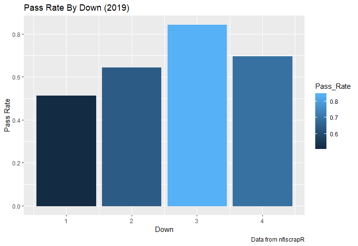
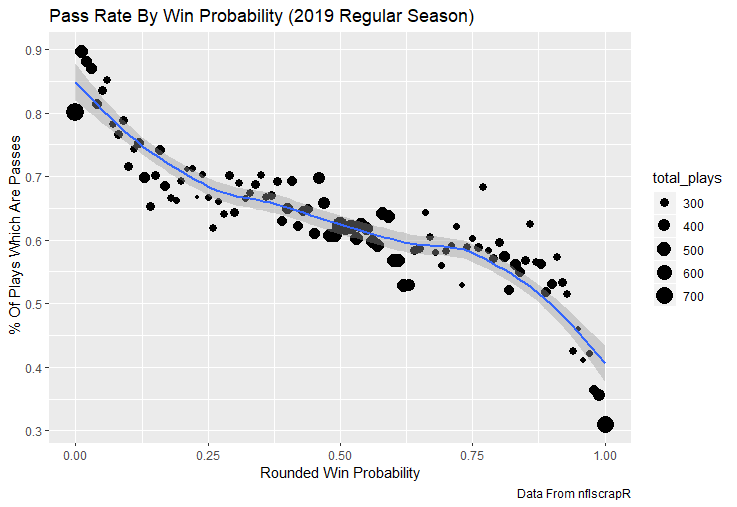
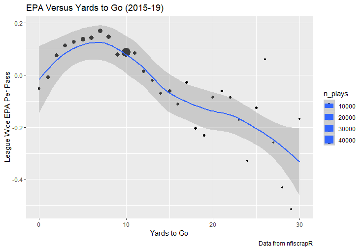
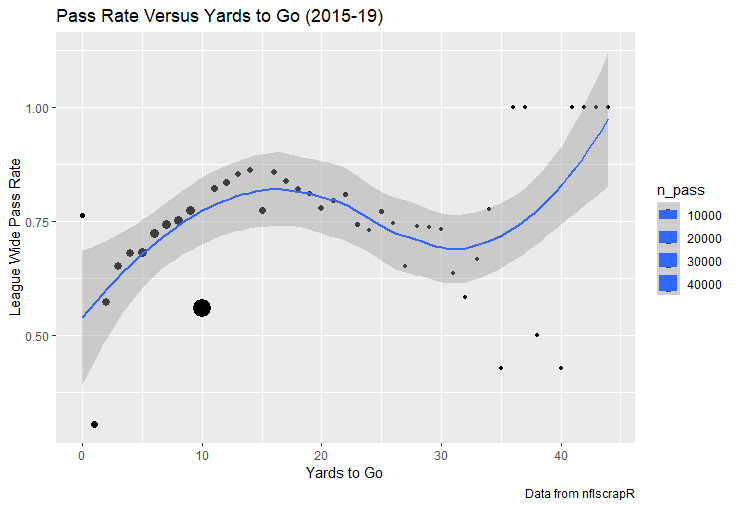
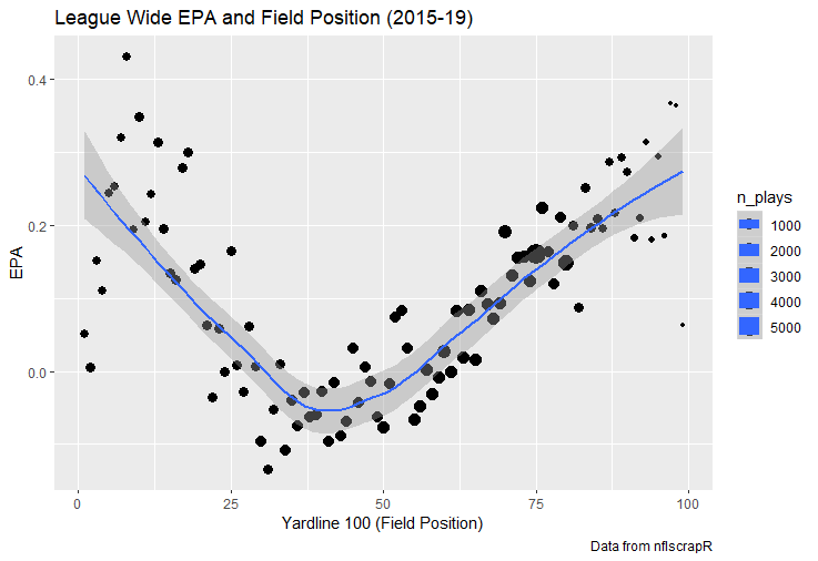
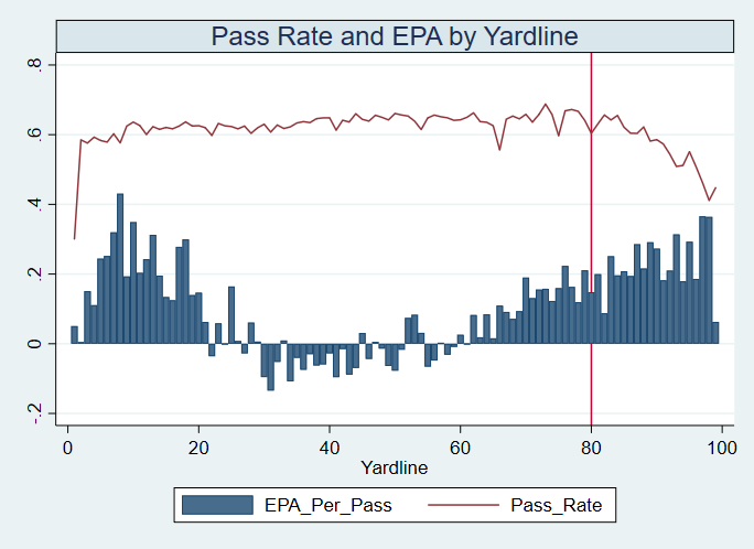
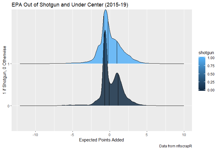
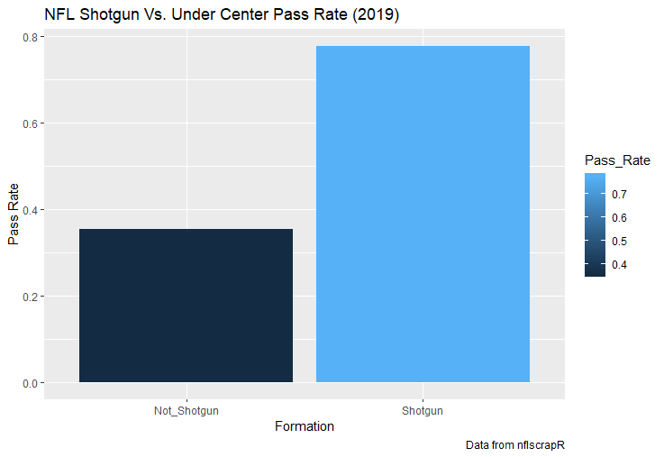
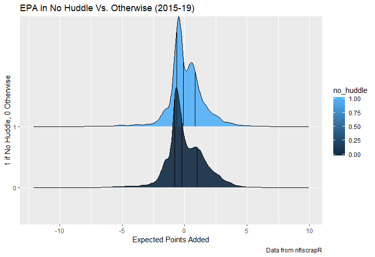
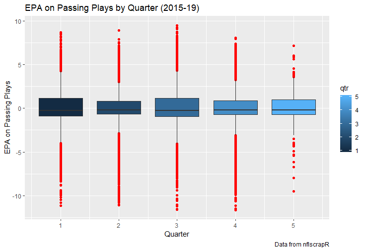
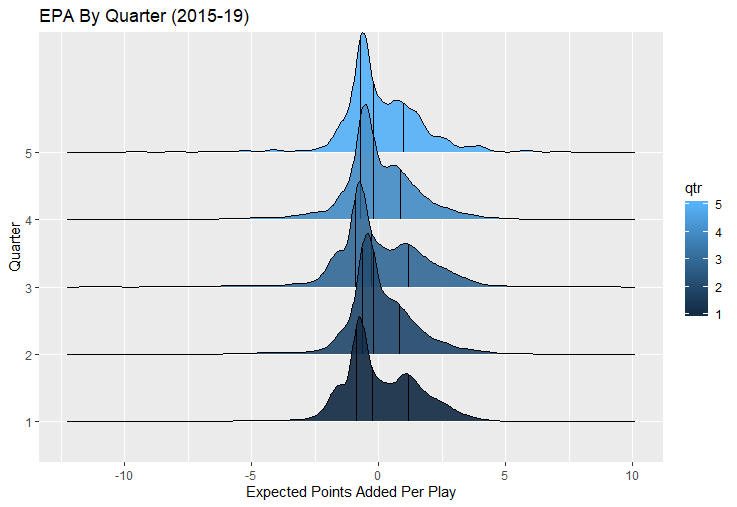
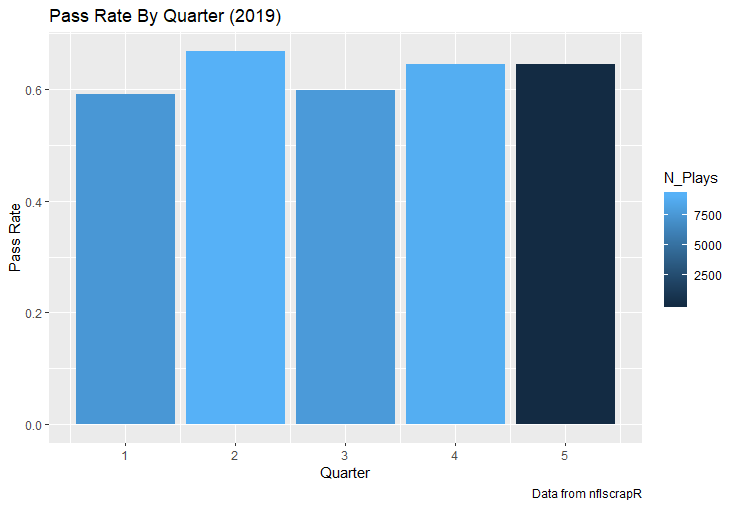
​For skill positions in the NFL like Quarterback and Running Back, production totals tend to largely be a product of opportunity.

As a result, efficiency measures like yards per attempt or Expected Points Added (EPA) per drop back are much better for evaluating players. Using NFLscrapR, it is easy to obtain these player statistics, but the same data set shows various things outside of the Quarterbacks control also affect these values. For example, all else equal, passing on first down tends to be more efficient than passing on later downs. Additionally, passing into 2019's number one ranked New England Patriots defence was more difficult than passing into the number 32 ranked 2019 Arizona Cardinals defence. If the goal of statistics is to aid player evaluation, adjustments should account for factors outside of a Quarterback's control. Thankfully similar adjustments have been made for years in hockey using Ridge Regression to create Regularized Adjusted Plus-Minus (RAPM)[1]. In the RAPM model, players go into a regression model as dummy variables along with control variables to estimate an individual's impact independent of other players and some contextual variables. This post will use the same concept and apply ridge regression to the NFL play by play data courtesy of NFLscrapR to obtain estimates of NFL Quarterback's EPA Per play independent of various factors in the dataset Quarterbacks have little to no control over.
[1] Macdonald, B. (2012). Adjusted Plus-Minus for NHL Players using Ridge Regression with Goals, Shots, Fenwick, and Corsi. Journal of Quantitative Analysis in Sports, 8. doi: 10.1515/1559-0410.1447

EPA and the Adjustment Idea
For a long time, offensive football statistics heavily relied on yardage numbers like yards per attempt (YPA). YPA is a useful starting point; however, any football fan knows not all yards are equally valuable. For example, show any fan or coach their team throwing a two-yard check down on first and ten, then they will be disappointed. However, show them the same two-yard pass on third and one, then the pass feels like a massive success. EPA tries to take this concept and weigh each play based on the expected value in terms of points it added relative to before the play. So, imagine a team in field goal range on second and nine from the twenty. Say under these circumstances teams end with an average of 4 points. Then the Quarterback hits a perfect pass right into the end-zone. The expected value of points on the drive increases from four to seven because they have now scored a touchdown. So, this pass is worth an EPA of three (7-4=3). Over enough passes, divide EPA by passing attempts to turn it into an efficiency measure. (Note most people here are likely familiar with Expected Goals in Hockey, you can think of EPA like xG for American Football, and this Model is like the Evolving Hockey's RAPM xG).

​The idea for this model came from a concept found in hockey analytics called “Score Effects,” and the RAPM. Gabe Desjardins discovered score effects when he realized the score state of the game heavily influences NHL shot rates[1]. In NHL level hockey, there is a counter-intuitive trend. The winning team is likely to control a smaller percentage of the shots, chances and goals than the losing team, and the effect gets even stronger as the score differential increases. So, on average, teams up by five goals are out-chanced by a larger amount than an identical team leading by one goal. The effect is likely caused (at least in part) by loss averse players and coaches, although perfect knowledge of the cause is not necessary to spot and adjust for the trend. The thought process behind this model was, if simple adjustments based on things like the score improve hockey statistics, they would likely do the same for football. There might even be potential for more significant improvement to NFL statistics because there are far more contextual variables in the NFL play by play data than the NHL. Each NFL play has 256 rows of data attached. Many of which likely impact the EPA on that play despite being out of the Quarterbacks control, like the defence, for example. The model being presented will try to account for these contextual variables a Quarterback has little to no control over, which will yield stronger estimates of the Quarterback's marginal effect on EPA per play.
[1] Desjardins, G. (2010, April 13). Corsi and Score Effects. Retrieved March 10, 2020, from https://www.arcticicehockey.com/2010/4/13/1416623/corsi-and-score-effects

Picking Control Variables and Adding Teams
​Using raw EPA data, Ben Roethlisberger had a terrible 2019 season. His -0.157 EPA per passing play ranked in the 18th percentile of Quarterbacks with at least 50 dropbacks in the 2019 regular season. A low EPA per pass is unlike Roethlisberger, who is usually one of the more efficient passers in the NFL. Upon closer inspection, it becomes obvious why he struggled so much in his small sample. He was injured for most of the year, so he only played one full game. That game just happened to be against the New England Patriots. Using the data set, we can see Roethlisberger’s EPA against the Patriots was far from unusual.

​Passing against the New England Patriots was incredibly difficult in the 2019 season. The gap between the Patriots defence and the league average was about 0.3 EPA per pass. For a player who throws 600 times in one season, this translates to an expected loss of 180 points relative to an average defence. The massive gaps between teams show why no players statistics should be used against them without first accounting for their quality of competition. To account for quality of competition, team variables are the first contextual factor put in the model. This was done by adding a dummy variable equal to one if that specific defence was the defending team. So, for example, the variable was_NE_D was set equal to one when the Patriots defence was on the field and 0 in any other game.

There is a bonus from team variables inside the model too. By including teams in the model, opponent and context adjusted efficiency estimates are obtained for defences too. This gives more robust estimates of team pass defence as well because the same things which affect Passers can also alter how efficient the defence appears. The same way players should not be punished for playing the 2019 Patriots; defences should not be punished for playing against 2019 Patrick Mahomes. 

​The next variables to go into the model were more difficult. The play by play data contains hundreds of variables, but you do not want to risk overfitting by including every single one. So, to decide which variables go in the final model, Lasso Regression was used on a dataset with all passing plays from 2015 to 2019 (a similar process to ridge regression, which the final model will ultimately use). Lasso is a type of regression that penalizes the absolute value of the coefficients towards zero. Lasso is helpful when choosing from many potential variables because it can set coefficients equal to zero and, therefore, remove them from the model if they do not help estimated out of sample predictions (determined using cross-validation). Lasso is not perfect or fully "objective", but letting Lasso pick the variables improve estimated out of sample error is probably better than me picking some significance level out of thin air, then running OLS on a group of variables, and including those that pass my arbitrary significance level. Before adding the variables into a Lasso regression to pick the models additional control variables, two variables had to be created first.

​Much like score effects in hockey, it was hypothesized the score of the game has an influence on passing efficiency. Better than raw score totals, NFLscrapR has win probability at the time of each play on the dataset. When comparing win probability to passing efficiency, the relationship does not appear to be linear.

​The relationship looks like it might be quadratic, so a win probability squared was added to the data-set. The next variable created was taking the log of yards to go. This variable is used in the EPA calculation, so it made sense to try it as a control variable in this regression. 

Next, it was finally time to run the Lasso regression, including the teams, players and then some ideas for control variables. The optimal model picked by minimizing estimated out of sample error included 9 contextual variables. Some were more obvious than others. The regression left out many players and teams whose coefficients were almost 0, but the goal is to evaluate all players and teams. So the players and teams Lasso left out were added back into the final model. 

Included Controls - Down
​The first variable added to the model was down. Teams like the Kansas City Chiefs were praised because they passed more often than anyone else in the league on early downs last season.

​Nerds praised Andy Reid and company for this because passing efficiency is negatively correlated with down.

So, imagine a cloned QB on otherwise identical offences, but the first team often passes on early downs like the Cheifs, and the second team generally preferred to run until third down. Then the Quarterback on the first more pass-happy team would have better statistics in the long run despite being identical to his clone, simply because of decisions his coach made.
​
Why does this correlation exist? There is no way to be sure, but it likely, at least in part, is because the defence can be increasingly confident a pass is coming as the down increases on the first three downs. (It is also likely in part just because of how the EPA calculation works)

Defensive coordinators are essentially flipping a coin between pass or run defence on first down, but by third down, they know a pass is coming almost 85% of the time. The more certain defensive play-callers can be of what’s coming, the better their players should preform all else equal. This is a possible reason why down is negatively correlated with passing efficiency and is therefore included as a control variable in this model.​
​
Win Probability Squared
The next variable added to the model was the squared win probability (Lasso dropped the linear win probabitly term). As seen before, the relationship between passing efficiency and win probability is probably quadratic. Again, this is likely because of how easy it is for defensive coordinators to predict what is coming next.

When teams are losing, they pass far more often than they run because passing is more likely to get them out of that deficit. On the contrary, teams generally play it safe and run when they are leading and likely to win so they can guarantee chewing some clock and do not have to risk interceptions. Defensive coordinators are therefor able to adjust and play pass first defence when the context calls for it, this is likely why passing efficiency is increasing as win probability does, because there should be a negative correlation between how likely a team is to pass and their efficiency when actually passing. It is easier to pass against defenses who do not see if coming. 
​
Yards to Go and Log Yards to Go
​​The third and fourth variable selected were yards to go and the created log yards to go. 

Pass to run ration likely does not explain this one though.

But, It is clear yards to go can affect passing efficiency, and the Lasso model selected both Yards to go and the Log of yards to go as a result. It makes an intuitive sense that teams far back from the chains struggle to add value. Teams can struggle enough to cover 10 yards in 3-4 downs, then once something goes wrong and they usually have 2-3 downs to make up 15+ yards they really struggle to add value in the passing game.

Yard-line 100 and Yard-line 100 Squared 
​Another field position variable was added after yards to go, called yard line 100 in the NFLscrapR data. This is where on the field the ball was spotted before the play. So, after a fair catch on kickoff, the team will be starting at their own 25-yard line, so the variable yard line 100 variable would equal to 25 for that pass. The yard line 100 variable has had a massive nonlinear effect on EPA per play since 2015.

Because of the way the relationship looks, a square term was added to the yard line 100 variable. As for the why, again this likely is not explained by disguising the pass from defenses. 

There is a weak negative correlation between the pass rate and EPA, especially once teams enter the redzone, but overall the relationship is not particularly strong between pass rate and EPA per pass by yardline. This relationship is more likely just caused by the EPA formula. It is presumably easier to add expected points from your own goal line, since the expectations are low. Or from there redzone where you are much more likely to throw touchdowns and guarantee points on the board. I am not means a football expert, so this could be explained by something missing from my analysis too. 

Shotgun 
The final two variables were more about the offensive scheme. The first is simply called “shotgun” and it is set equal to one if the offence comes out in shotgun formation, and zero otherwise. Teams generally go to shotgun formations to pass, so it is easy to assuming that is because passing out of the shotgun is more efficient than under center, but the opposite is true. NFL teams have been less efficient when passing out of the shotgun.

The relationship does not pop off the page to the eye, but it is consistently a negative coefficient. Why is passing out of the shotgun less efficient when teams generally go to the shotgun specifically to pass? Without experience playing Quarterback this can be tough to answer, but again it probably has something to do with team’s tendencies given this information.

Teams pass out of the shotgun about 80% of the time but pass less than 40% of the time otherwise. Again, this should make it easier for defenses to prepare since the offence’s formation is a key tell of what might be coming. Additionally, a friend of mine who played Quarterback mentioned he preferred passing from under center because routes tended to take longer to develop out of shotgun formations. This meant defensive backs were better at jumping routes when passing from the shotgun. That is just one guys thoughts but I found them interesting. Either way passing out of the shotgun has tended to lower passing efficiency in the NFL, all else being equal. Therefor it would be unfair to punish players for their coach calling shotgun passes more often than some other teams’ coach. 

No-Huddle 
In a similar vein, there is a variable called “no_huddle”. This dummy variable is set equal to one if the offence runs a hurry up and does not huddle and is equal to zero otherwise. NFL teams have been more efficient when passing after running a no huddle.

Intuitively, if defences are given less time to prepare, they should be worst at defending the pass, and that relationship holds. Score one for the air raid. It is not a major difference, but again a Quarterback can have their EPA per pass increased because their coach calls a no huddle offence more often than some other Quarterback’s coach, and this variable will account for that.

Quarter 
​The final relationship is the negative correlation between the Quarter of the game and EPA per play

The reasoning is much more ambiguous here. I figure many variables have their correlations because it is a tell to the defence of what is coming, but that doesn't seem likely for Quarters.

 Not only is the relationship less obvious to the naked eye and hard to explain, it is least statistically significant. That being said the variable was consistently picked by the Lasso model. Maybe defense's are better at adjusting to the offence in game than the reverse? I'm not entirely sure to be honest.

Altogether this leaves the model with nine control variables

1. Down
2. Yards to Go
3. Log Yards to Go
4. Yardline 100
5. Squared Yardline 100
6. Squared Win Probability
7. Quarter
8. Shotgun
9. No Huddle

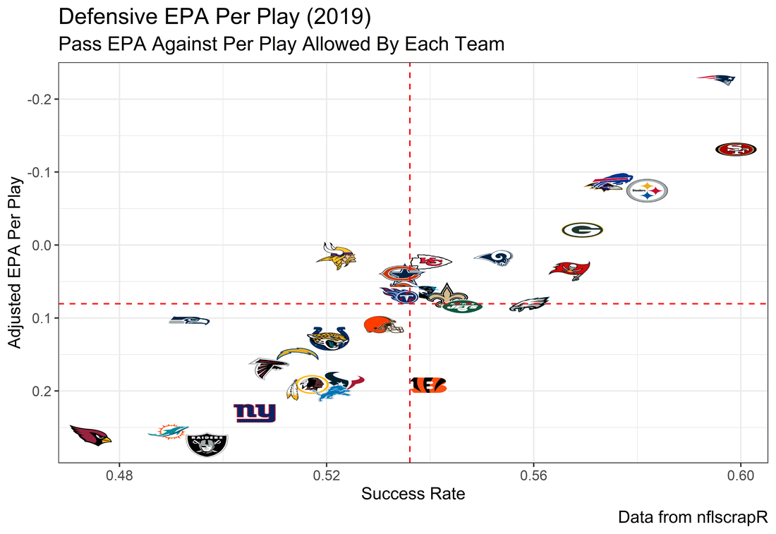
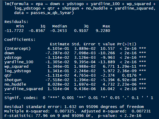
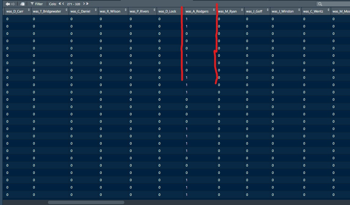
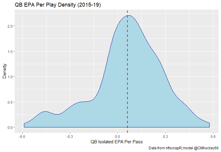
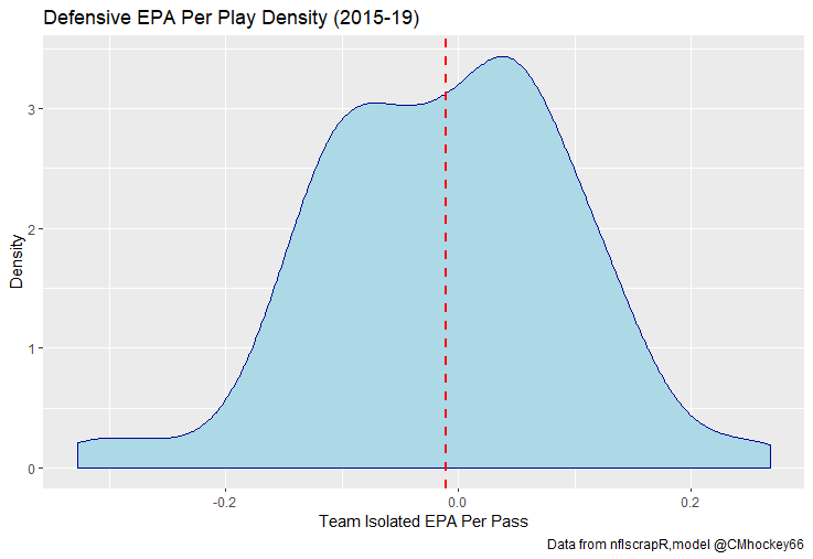
​The goal of using lasso regression to pick the variables was to rely on something other than picking some significance level and looking at P values, but all these variables end up being significant at the 2% level anyways. (Data from 2015-19)

Adding the Quarterbacks
The final piece of the puzzle is adding in the Quarterbacks themselves. Just like adding the team variables, the Quarterbacks go into the model as dummy variables. So to obtain estimates for Tom Brady, a variable called “was_T_Brady” was created to which is set equal to one if the passers name was “T.Brady” in the play by play data. Here's a look at what this looks like in R added on to the play by play data. For those of you familiar with the Evolving Hockey RAPM write-up, this might look familiar to you. 

​The first game in the 2019 play by play data was between the Green Bay Packers and Chicago Bears. So as you can see Aaron Rodger's passing variable is set equal to 1 for many of the first passes. Once a variable is created for each passer and the contextual variables are created the model is ready to go. An additional note is that I chose to run the model filtering out three key things.

First being two point conversions. Down is a control variable, and not really available for two point conversions so it was left out by filter to down != "NA". Next was passes where the passer's name was not available. For whatever reason the name of the passer is missing from like one thousand passes each year, maybe these are double passes or something. Either way those are filtered out. Finally only Quarterbacks with at least 50 passes were included. Evaluating the Julian Edelman's of the world who throw two passes or whatever per season is not the point of this model. Its goal is to evaluate actual Quarterbacks, and filtering out those who have thrown fewer than 50 passes is a good way to eliminate gadget type players. The final reason is too help not including players who have only thrown passes against one team. There is little to no point in estimating a player who only threw against a single defence, so this was an way to avoid doing so. Now that the data is all set, it's worth looking at what kind of model we are choosing and why.

​Ridge Vs. OLS
Obtaining player estimates while holding various contextual factors constant may sound like a job for OLS regression, but there are a few key advantages to using a ridge regression model. Ridge works similar to OLS, however the absolute values of the coefficents are penalized, just like in the Lasso model above. Difference with Ridge is the coefficients are penalized asymptotically close to zero. This means every pararmeter fed into a ridge regression model has an estimated value, none are removed. The penalization is done with a tuning parameter called lambda. The larger the lambda the larger the penalty. Like the Lasso model, the optimal Lambda was selected using cross validation in the glmnet package in R. The lambda penalization adds some bias to the model in order to reduce the variance. In theory, ridge models work best when you know all the variables are important beforehand. In reality this is usually useless theory because you cannot know what the important variables are beforehand, but sports analysis can be an exception to that rule. Sure, Tom Brady and Andy Dalton did not have a statistically significant difference in their production last season, but it is still clear to sports analysts Tom Brady is not Andy Dalton. 

​As a result, they can both go in a model like this one as variables. Other fields probably almost never have this advantage, but sports nerds do. ​

​Additionally, penalization tends to make Ridge regression better at estimating when variables are highly correlated. So, for example Ben Rothslisberger throwing most of his passes against New England last season means the variable was_B_Rothslisberger was highly correlated with was_NE_D in the 2019 dataset. OLS tends to struggle in these situations more than ridge regression.
​
Finally, using dummy variables for players and teams makes OLS estimates very difficult to interpret from year to year. Running a regression with dummy variables in OLS is done by leaving one of the variables out to avoid perfect collinearity. You then interpret the remaining variables as the marginal effect relative to the variable which has been left out. So say of the 32 defences, the variable for the Patriots defence was left out, then every team would be estimated as having a positive effect on EPA per play (Defences would try to be as negative as possible). Not because every defence in the NFL was bad, but because they were all worse than the Patriots. This is not the worst thing for one season but comparing the 49ers defence in 2018 to 2019 would be saying something like “Relative the Miami Dolphins defence in 2018 the 49ers defence lowered EPA per pass by 0.1, suggesting they were a good defence. Then they improved in 2019 by subtracting 0.3 off EPA per pass relative to the Dolphins”. The obvious question becomes How much does a team need to beat the Dolphins by to be good? Did the 49ers get better or did the Dolphins get worse? Some combination of both? If so, how much of the defensive improvement was the actual 49ers defence and how much was the Dolphins getting worse? These questions may be tough to answer. Worse yet, if the Dolphins happen to be the team left out, its even more difficult to interpret their marginal effect on passing efficiency. This makes interpreting an OLS with so many dummy variables difficult. On the other hand, ridge can obtain estimates for all 32 teams within the same regression. 

Results
Now for the fun part. First we can look at the most efficient starting Quarterbacks from last season, after adjusting for our contextual factors. I've never used the slideshow feature on Weebly before, but hopefully you can click through these charts to the a viz of starting QBs efficiency for each of the past 5 seasons. (Note the 32 QB's with the most passes thrown were included so the chart is actually interpretable, if your looking for the full data-set you can get the google doc here).

For those interested in the defensive side of the ball, here are are the adjusted defensive EPA per play coefficents.  

It is easier to see the effect the adjustments have on defence. The Patriots lapped the field in raw EPA per play against, but they also had a surprisingly soft schedule. As a result our adjustments push the Pats down to 2nd place behind the San Fransisco 49ers for hardest defence to pass against last season. Also of note the Cheifs rise from that mushy middle of the pack to the 4th spot. 

Here are the distributions. For QB's.

And the same for defences

Discussion
The entire point of EPA is to weigh specific contexts differently than others. This model kind of pushes EPA analysis in the opposite direction, so I suspect there may be some push-back there. Ultimately I think it depends on what you're using the statistic to evaluate. People generally use statistics to evaluate players. I mean, who doesn't love a good fight between Ben Baldwin and Packers fans about how Aaron Rodger's EPA per play in the past few seasons suggests he's overrated. Assuming this is the goal of using statistics such as EPA per play, this model should be helpful. If you want to be using statistics to evaluate player performance, a good faith attempt to estimate what portion of a player's statistics he is actually responsible for is essential.

Not that this is a perfect way to isolate for context. Nor do I think this model is complete and finished. I am not perfect at working with the data we have publicly, and there is plenty more non-public data such as wide receiver quality and O-line play not being accounted for in the model. But more generally, if you are going to using EPA to suggest a Quarterback is of ______ talent, you don't want EPA to be swayed by what formations the coach is calling, and what team the QB is playing against, because they can be punished (or praised) for things outside of their control. We know various things affect QB performance, this is why people talk about stats "not including garbage time" on Twitter where they filter out blowout games (Win prob above 80% or below 20%) because statistics in these contexts are less indicative of true talent. Filtering out garbage time makes some sense. Hockey did this too at first. They started by looking at "Corsi Close" where they only evaluated teams when they were within 3 goals of the other team. After a while, it became apparent throwing away that much data is unwise. In the 2019 NFL season, 18044 of the 45546 plays in the play by play data, or just about 40% the season came in this "garbage time." And unfortunately, no amount of fancy math compensates for lack of sample size, so simply throwing away that much data is unwise. This means the natural next step is adjusting the numbers based on the context rather than throwing out some of the limited information we have. Hopefully, this model is a step in that direction for Football analysis.

Next Steps
There are a few next steps I have in mind. First is to apply the same thing to the run game. Passing is more important, more interesting to me, and more likely to have actual signal in the results, so I started there. That being said, there might be some value in trying the same thing for the run game, and there is only one way to find out. After that, I would like to create a model predicting the probability any given play will be a pass as a control variable. This is a more direct way of adjusting for something I suspect the model is already doing. Other than that, I'm all ears. I didn't grow up a Football fan all my life, maybe there is something more experienced fans think I'm missing or stupid for doing in this model, and if so I'm all ears @CMhockey66 and [email protected]. If you have any ideas for improvements, general questions comments or concerns I'd be happen to listen or try and help. In fact this post is essentially the rough draft for a paper due in early April, so improvements are even more welcomed. Finally shoutout to this NFLscrapR intro, plus the RAPM model on Evolving Hockey for the idea behind using players as dummy variables in a regression model. Plus the Twins at Evolving Hockey for helping me with my questions when working on this each time I asked. And if you made it this far, thanks for reading!