|
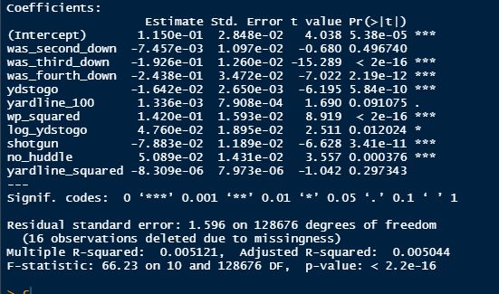
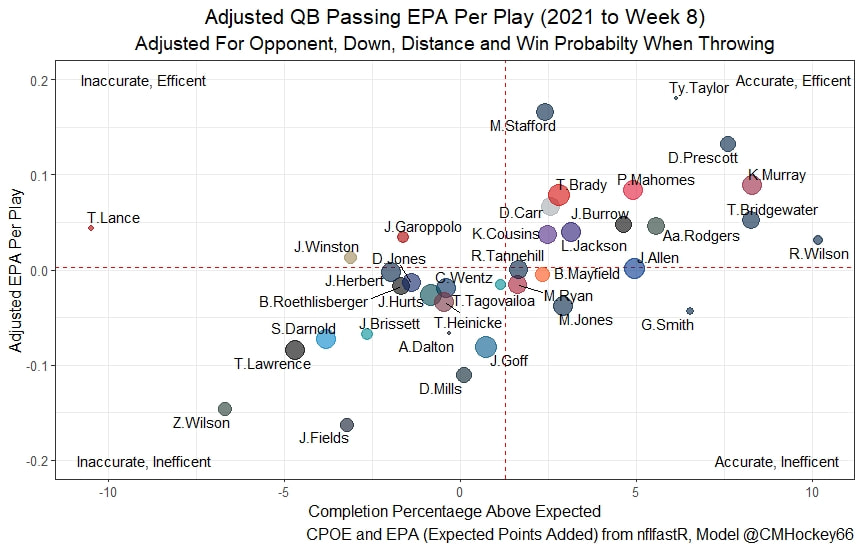
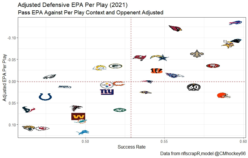
This post is going to reintroduce a model I created to evaluate NFL Quarterback and Defense's. For now I am calling the metric "Adjusted EPA Per Play". What this metric does is takes Quarterbacks Expected Points Added (EPA) numbers, and calculates them independent of the defenses they have played, plus the down, distance, field position and win probability at the time of their throws. The inverse of that is it also allows us to see defensive EPA per play estimates independent of quarterbacks, plus all those contextual factors. This is not a finished project. I first created this a few years ago for a school project, and have been testing it recently with all the signs being encouraging so far. It is still early in the testing phase, but I wanted to get something out there as a sort of proof of concept that would also allow me to get feedback from other people. This way I can make adjustments if need be before fully testing the model, and releasing it. So, lets dive in. I am going to start with a quick explainer of where this idea came from in case that interests you, if you just want to see the metrics writeup feel free to skip this first part. 1) Why Adjusted EPA? A Hockey History Lesson I am a hockey analytics nerd with a secondary interest in NFL football and its stats community. Note for my hockey nerds reading, you can think of EPA like Excepted Goals in hockey. But, when scrolling through football stats tweets, I noticed a familiar theme. The first was that football people sometimes filter out "garbage time". This is only using stats while the game is at least somewhat close because somebody putting up big numbers while up 37 points probably isn't that meaningful. Hockey nerds noticed a similar problem some time ago, calling it score effects (winning teams to get outplayed in hockey, once winning). What nerds who came before me first did was look at "Corsi close". This was the same thought process as football analysts filtering out garbage time, where Corsi close only included stats from when the game was within 3 goals. But, what hockey analysts have done since is "score adjust". They have found that rather than filtering out good some of our precious data, it is better off to adjust for the score of the game. When doing so, you have a larger dataset, and therefore your variables are more predictive. So I figured something along the same lines could be done for Football. I figured rather than filtering out garbage time or only looking at early downs or something like that, it might be a good idea to create an adjusted metric for football too. These metrics could make better predictions, along with being more descriptive (assuming you want to know a quarterback/defence's marginal effect on EPA per play, not just how efficient the offence is when they are throwing/being thrown against). To make such an adjustment I decided to make a ridge regression model. This would allow us to estimate all of the quarterbacks and defenses effects on EPA that season, independent of each other the various contextual variables we know affect outcomes. For example, if one team doesn't throw enough on early downs, the QB's raw EPA numbers will be punished, but an adjustment should help us better compare QBs across different contexts. Now let's dive into the model. 2) Why Ridge Regression The basic idea is to program a dummy variable for each team and defense. This variable will be equal to one in the NFLfastR dataset when that QB is throwing the football, and when that defense is on the field. So, when Tom Brady threw against the New England Patriots, I literally made my variables named "was_NE_D" and "was_T_Brady" for was New England's defense and was Tom Brady throwing the football, and these variables were each equal to one. Every other defense and QBs variable was set equal to 0 in this scenario. Then the next week when Brady is playing against a new defense, his variable and that new teams dummy variable will be set equal to one. It is tedious as hell, but a dummy variable must be created for each QB who throws a pass, even the Julian Edelman's of the world who pass like twice a year, plus each defense. Then, put all the QB and team dummy variables, along with a handful of other control variables into a ridge regression model together, we get opponent adjusted QB and defense EPA per play, that also accounts for all the other variables in the model. My idea to use Ridge Regression came from Evolving Hockey's RAPM model, which they based on an old research paper by Brian Macdonald, which he came up with based on a Basketball statistics. In other words, using ridge models to isolate performance from opponents and contextual factors is not new in sports. Ridge is works like OLS but the values are penalized towards zero by a factor called lambda. The benefit of using a ridge regression model for this analysis is it allows us to obtain estimates for every team and defense in the NFL. With OLS we would have to leave out one QB and one defense, so the coefficients would get really, really hard to interpret, especially year over year. Additionally ridge tends to preform better than OLS when there is a high degree of collinearity between variables, I don't believe this problem (given our current set of play by play data) is as much of an issue for football as hockey/basketball, but it definingly should improve the model when dealing with smaller samples than a full season. The downside of ridge is that there are no standard errors, since the coefficients are penalized towards 0. Note I have run this model with a lasso instead of a ridge model before, but a lot of QB and defense estimates are simply set equal to zero using lasso. I believe it is far, far more interesting to obtain estimates for each player. With the model set, and a dummy variable for each quarterback and team created, let's move on and look at the control variables selected for the model. 3) Control Variables Down - The first and most obvious control variable is the down. NFL nerds always talk about how throwing on early downs is more efficient than throwing on late downs. As a result, they praise teams who pass more on early downs. The one problem with the differences in down to down efficiency is when evaluating quarterbacks, a players efficiency statistics can be artificially inflated by his offensive coordinators run pass balance on early downs. So, by including a dummy variable for each down set equal to one when that down was thrown on, we allow a flexible estimate of down to down efficiency, and get the QBs EPA per play independent of how often he passes on each down. Yards to Go - The next variable is yards to go for a first down. Throwing with more yards to go has tended to be more difficult for quarterbacks. This makes an intuitive sense, it is more difficult to come up with a positive play when you need 10 yards than when you need 1. So I included a control variable for yards to go. I also noticed a non-linearity and added a log term along with yards to go. This was from when I originally created the model, I am not sure this is the optimal way to account for this, so if you have any better ideas please let me know. Shotgun - NFLscrapR and its younger brother both include a dummy variable set equal to 1 if teams are in the shotgun formation (For hockey nerds this is when the QB is standing far being his center and takes the snap through the air, teams usually do this when they are passing). Passing out of the shotgun has been less efficient in every iteration of this model that I have created, and it seems to be out of the QBs control. So, we will be adjusting for that as well. No Huddle - On the contrary, passing after running no huddle has been more efficient. This makes sense that it helps the offence more than the defense because the offence is the one who gets to chose when and when not to run no huddle. So, this variable will also go into the model. Win Probability - This one is inspired by score adjusted numbers in hockey, and Football people filtering out garbage time. Passing seems to be more and more efficient at really high win probabilities, and difficult with low win probabilities. As a result, a win probability term was included in the model. Note there also appeared to be a nonlinearity here, so a square term was added as well. Open to suggestions on if this is actually optimal or not. Field Position - The final variable included in the model is accounting for field position. It appeared although some areas of an NFL field are more difficult to throw from, so I included this variable originally. It appears although the significance of this variable in the model has declined in recent years, so I may stop accounting for field position in future iterations. Note that I used both a linear and squared term here too. So with all these variables selected, I will show you a quick regression when filtered to only look at passing plays since 2015. Here we can see that these control variables (other than that field position one) have statistically significant effects on EPA per play. Furthermore we know that different QBs face these variables at different rates. So this model should help us better judge QB and team (pass) defense efficiency by controlling for all these variables. Results There are a few ways to look at the results. The first is that we can look at estimates within the current season. These in season estimate charts should look familiar to football fans. At this point in the season the biggest benefit is probably accounting for opponents. This model allows us to do so, even in season. It can be interesting to note the biggest risers and fallers relative to unadjusted EPA per play. After accounting for context, the model really likes Dak Prescott, Kyler Murray, and Derick Carr. On the flip side, the adjusted numbers are less kind to Mac Jones, Jameis Winston and Josh Allen. As for defenses, the model really likes the Cardinals and Chargers, while being lower on the Chiefs and Raiders. The other way to look at the results is to watch them over time. Note I mentioned before this is only the beginning of this model, and its time consuming to get estimates for a season because each passer requires a variable in the model. As a result, the numbers only go back to 2017 right now, but we can still look at the 5 most efficient seasons by defenses and quarterbacks.
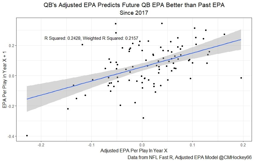
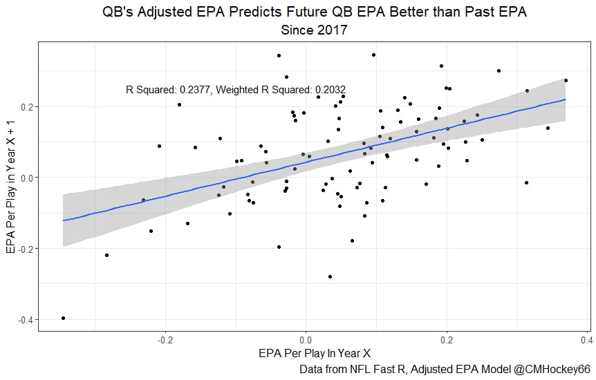
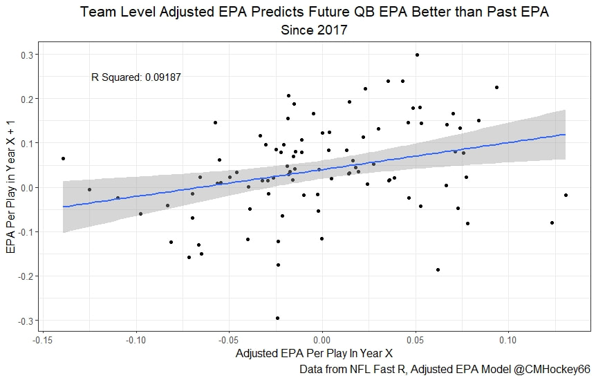
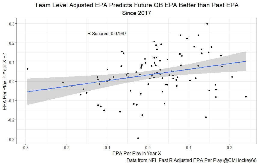
All the MVPs and historic defense's show up just like with EPA. Only thing to note is that for those used to working with EPA data, the adjusted EPA per play estimates are much smaller than the unadjusted EPA numbers. So What? Anytime a new metric is released, the first question anybody should ask is so what? And honestly, this can be a difficult question to answer. For a new metric to be useful, it should probably be either more descriptive, or more predictive than existing metrics (or some combination of the two). Since my metric is built off EPA, the obvious benchmark will be comparing it against EPA. If a metric is more descriptive or not seems somewhat nebulous, but I do believe this metric is a better description of a Quarterback / defenses impact on expected points added because it accounts for various contextual variables. This is especially true for defenses because of the opponent adjustment. If smart people like Eric Eager are right (and they probably are), then a defense is more heavily influenced by the QB they play than their own talent. As a result, EPA per play that accounts for the opposing QB should be incredibly helpful. Then there is the predictive value than previous metrics. Specifically for adjusted EPA per play, let's look at and see if it is more predictive of future EPA per play than unadjusted EPA per play. First we can look from the QB perspective. This will be done by looking at year over year correlations. Note that the "weighted r squared refers to running the year over year regression weighted by the total number of dropbacks the QB had over the two year period. While the difference is small, a QBs adjusted EPA per play is actually more predictive of future EPA than his past EPA per play. Next we will see the same is true for defences as well. So overall, its still early, but all the signs are positive. I believe the metric makes sense in theory, descriptively, plus it seems to be slightly more predictive than past EPA at the team and player level. Additionally, this metric is more repeatable than raw EPA per play (ie its more predictive of itself year over year than raw EPA is) , again using the weighted and unweighted regressions we get an R squared of 0.2679 and 0.2396. While this is not a massive difference nor a huge dataset, these are the most positive signs I could realistically hope for. Again, testing is not complete, I would like some feedback from people in the football stats community, but the signs are all positive thus far. If you have any questions, comments or concerns, feel free to reach out to me on Twitter, @CMhockey66!
0 Comments
Leave a Reply. |
AuthorChace- Shooters Shoot Archives
November 2021
Categories |
 RSS Feed
